6 Storage

This section will give provide SOP for key technologies within our infrastructure

Parquet
HDFS local and server
HDFS Cloud

6.1 Parquet

Apache Parquet is a columnar storage format that is optimized for modern analytics. It is the foundation of modern analytics technologies such as Open Table Formats, OLAP data engines and high performance distributed computing such as Apache spark. Please refer to this chapter in R4DS for a more hands on introduction. Here are some of the benefits

Column data types are retained as metadata
- Column data type is stored so you don’t have to worry about parsing integrers, strings, dates that get lsot in .csv files.
Efficient storage:
- Data is stored in a highly efficient way so file sizes are many folds than other storage formats
Efficient analytics
- Format optimized for big data queries
- Effective for distributed computing
Open source
- high iteroperability with modern data tools (Arrow, OLAP engines)

We can work with parquet in many languages (R, Python, JS, Rust, C++ … etc) with the Apache Arrow package.

6.1.1 1. Export tabular data as parquet

Here lets geernate some data and save it a parquet.

## Load packages
library(tidyverse)
library(arrow)

## Simulate data
set.seed(123)
n_rows = 100000
data = tibble(
  id = 1:n_rows,
  name = sample(letters, n_rows, replace = TRUE),
  value = rnorm(n_rows),
  race_ethnicity = sample(c(1:3), n_rows, replace = TRUE),
  date = sample(seq(as.Date('1999/01/01'), as.Date('2000/01/01'), by="day"), n_rows, replace = TRUE)
)

## EDA
dim(data)

[1] 100000      5

head(data)

# A tibble: 6 × 5
     id name   value race_ethnicity date      
  <int> <chr>  <dbl>          <int> <date>    
1     1 o     -0.285              1 1999-01-12
2     2 s      0.381              2 1999-02-15
3     3 n      1.20               3 1999-03-23
4     4 c      1.08               1 1999-04-05
5     5 j      1.05               1 1999-10-10
6     6 r     -1.62               1 1999-07-13

Now lets write this data to our local storage both as .csv and parquet.

arrow::write_parquet(data, "data.parquet")
write.csv(data, "data.csv")

Notice how the parquet file is much smaller than the .csv file. This is because parquet is a columnar storage format and is optimized for efficient storage and access.

6.1.2 2. Import .parquet tabular data

Lets import the parquet and make sure all of our metadata is retained.

df_import = arrow::read_parquet("data.parquet")
head(df_import)

# A tibble: 6 × 5
     id name   value race_ethnicity date      
  <int> <chr>  <dbl>          <int> <date>    
1     1 o     -0.285              1 1999-01-12
2     2 s      0.381              2 1999-02-15
3     3 n      1.20               3 1999-03-23
4     4 c      1.08               1 1999-04-05
5     5 j      1.05               1 1999-10-10
6     6 r     -1.62               1 1999-07-13

Notice how our original column types integer, character, double and date are all retained. This feature really helps data teams work effecitevly without having to worry about type casting getting lsot in translation.

6.1.3 3. Column type metadata

We have touched on one of key benefits of parquet which is the retention of metadata - such as column data type (e.g. int, string, date). But we can also store a lot of other metadata in our parquet files include spatial metadata (Coordinate systems) or even custom metadata such as column definition or column coding. Lets demonstrated this with the data we imported above. Lets demonstrate this with the data we created above.

First lets convert it into arrow table format.

arrow_table1 = data %>% arrow::arrow_table()
arrow_table1

Table
100000 rows x 5 columns
$id <int32>
$name <string>
$value <double>
$race_ethnicity <int32>
$date <date32[day]>

we can see the column types are strictly retained. But we could also change the metadata which in Arrow is called the table schema manually. Lets update two column types to adhere to best practices:

id
- old: integer
- new: string
- Why: ID’s are commonly stored as a string instead of integer
name
- old: string
- new: utf8
- Why: column is curently just a string but its good to specifically specific string UTF-8 encoding for complex names (e.g diacritical marks).

Below we define the new schema and update our table.

## Update data
data2 = data %>% 
  mutate(
    id = as.character(id)
  )

## Define new schema
new_table_schema = arrow::schema(
  id = string(),
  name = utf8(),
  value = double(),
  race_ethnicity = arrow::int32(),
  date = arrow::date32()
)

## Update the table's schema
arrow_table2 = arrow_table(
  data2 ,
  schema =new_table_schema
)
arrow_table2

Table
100000 rows x 5 columns
$id <string>
$name <string>
$value <double>
$race_ethnicity <int32>
$date <date32[day]>

We can see the table’s metadata has been updated! We can save this as a parquet and now all downstream users will have this metadata automatically imported and have the correct column types. In addition to column type we can store almost any type of metatdata in parquet, please refer to the Parquet Metadata Documentation for details. Below we explore two common use cases for custom metadata: 1) embedding column definitions and 2) embedding categorical coding information.

6.1.4 4. Custom Metadata: Dataset and column

Here we follow R Arrow’s metadata documentation to demonstrate how to embed column definitions in a parquet file and how uses can access this built-in codebook. Essentially we when a data.frame is converted to an Arrow table which can be saved as parquet, any attributes() attached the columns of the original data.frame is also converted and saved.

Lets first initialize our example data.frame

## Initialize our demo data.frame
data3 = data %>% 
  mutate(
    id = as.character(id)
  )

6.1.4.1 4.1 Dataset level metadata

We can append dataset level metadata as custom key value pairs.

## Dataset description
attr(data3, "description") <- "A simulated dataset for demonstration purposes."

## Author
attr(data3, "author") <- "Harry Potter"

## Author ORCID
attr(data3, "author_orcid") <- "https://orcid.org/0000-0002-9868-7773"

Lets check that this information is retained in our Arrow table.

arrow_table(data3)$metadata$r$attributes

$description
[1] "A simulated dataset for demonstration purposes."

$author
[1] "Harry Potter"

$author_orcid
[1] "https://orcid.org/0000-0002-9868-7773"

6.1.4.2 4.2 Column level metadata

It is also very useful to be able to write custom metadata at each column. In this example we will annotate our race_ethnicity column which is stored as integer for efficient processing but low acecssibility. Lets enrich this column with metadata to make it more accessible to users who get this file.

## Column description
attr(data3$race_ethnicity, "description") <- "This column represents race and ethnicity"

## Column Coding
attr(data3$race_ethnicity, "coding") <- '1:White, 2:Black, 3:Hispanic'

Lets check that this information is retained in our Arrow table.

arrow_table(data3)$metadata$r$columns

$id
NULL

$name
NULL

$value
NULL

$race_ethnicity
$race_ethnicity$attributes
$race_ethnicity$attributes$description
[1] "This column represents race and ethnicity"

$race_ethnicity$attributes$coding
[1] "1:White, 2:Black, 3:Hispanic"


$race_ethnicity$columns
NULL


$date
NULL

We can see that the column metadata is retained! Just to be sure lets save this an re-import to make sure our metadta is intact

## Write
data3 %>% write_parquet("data_with_metadata.parquet")

## Import  
df_import = arrow::open_dataset("data_with_metadata.parquet")

## Check
df_import$metadata

$r
$r$attributes
$r$attributes$description
[1] "A simulated dataset for demonstration purposes."

$r$attributes$author
[1] "Harry Potter"

$r$attributes$author_orcid
[1] "https://orcid.org/0000-0002-9868-7773"


$r$columns
$r$columns$id
NULL

$r$columns$name
NULL

$r$columns$value
NULL

$r$columns$race_ethnicity
$r$columns$race_ethnicity$attributes
$r$columns$race_ethnicity$attributes$description
[1] "This column represents race and ethnicity"

$r$columns$race_ethnicity$attributes$coding
[1] "1:White, 2:Black, 3:Hispanic"


$r$columns$race_ethnicity$columns
NULL


$r$columns$date
NULL

Indeed this metadata is retain in the parquet file.

6.2 Out-of-memory computations

One major benefit of modern analytics is the ability to work with datasets larger than a computer can load. Lets demonstrate how we can work with our data.parquet file without laoding into memory; importantly, this workflow scales and will alow analysts to easily work with datasets in the 10’s, 100s of GB or even Terrabyte sized datasets on normal labtops.

The first step is not to import the data but rather to connect with the data.

dataset = arrow::open_dataset("data.parquet")
dataset

FileSystemDataset with 1 Parquet file
id: int32
name: string
value: double
race_ethnicity: int32
date: date32[day]

Notice how when we print the dataset object we don’t get a table but rather a abstraction called a FileSystemDataset and the metadata of the data inside this abstraction.

We can now run write our data wrangling logic and compute on this dataset without loading it into memory. For example here we write normal dplyr code - note that Arrow supports many data wrangling API’s such as python pandas or Rust Polars and many other languages.

dataset %>% 
  filter(date > as.Date("1999-12-31")) %>% 
  mutate(id_name = paste0(id, name)) %>% 
  collect()

# A tibble: 272 × 6
      id name    value race_ethnicity date       id_name
   <int> <chr>   <dbl>          <int> <date>     <chr>  
 1   441 k      0.111               3 2000-01-01 441k   
 2   769 t      2.87                3 2000-01-01 769t   
 3  1259 e     -1.43                3 2000-01-01 1259e  
 4  1280 z      1.02                2 2000-01-01 1280z  
 5  1901 u      0.161               2 2000-01-01 1901u  
 6  2168 c      0.467               3 2000-01-01 2168c  
 7  2690 q     -0.854               1 2000-01-01 2690q  
 8  2721 o      1.13                1 2000-01-01 2721o  
 9  3224 z     -0.0604              2 2000-01-01 3224z  
10  3632 n      0.386               1 2000-01-01 3632n  
# ℹ 262 more rows

6.3 File systems on Server

In addition to working efficiently and out of memory with a single file. We can partition how we store our files to accommodate the operating parameters of our hardware but also enable users to access the data not piece wise but as an single file system.

Add more details here and show some schematics

For example we have stored the CCUH PRISM zonal statistics as an HDFS. Here an analyst can access this entire resource both get the data thye want but also to run some basic data operations. Importantly, this allows us to utilize existing infrastructure such as the access controled drexel Servers.

Lets connect to the PRISM Zonal Statastics HDFS.

server_prism_path = '//files.drexel.edu/colleges/SOPH/Shared/UHC/Projects/PRISM/SAM/processed/hdfs_prism_results'
dataset = server_prism_path %>% arrow::open_dataset()

dataset

Lets just get a rough idea of how much data is in this dataset in terms of measure, year, geographic level.

dim(dataset)
dataset %>% 
  select(geo_level, measure, year) %>% 
  distinct() %>% 
  count(geo_level, measure) %>% 
  collect()

So this data current is jsut for the state of PA and contains 161 million rows. with 5 geographic levels and 5 measures and 13 years of data. In .csv of other formats this would be many GB but we can access it quickly and only pull into memory the data we want.

For example an analyst wants to pull all tracts in Philadelphia for all measures and years.

## Get a list of Phialdelphia Census tracts
library(tidycensus)
tracts_philly = get_acs(
  geography = "tract",
  variables = "B01001_001",  # Total population variable (used just to retrieve tracts)
  state = "PA",
  county = "Philadelphia",
  year = 2020,
  geometry = FALSE  # Set to FALSE since we only need GEOIDs
) %>% pull(GEOID)

## Query our dataset
df = dataset %>% 
  filter(
    geo_level == "tract10", 
    measure == 'tmean',
    GEOID %in% tracts_philly) %>% 
  collect()

head(df)

6.4 File Systems on Cloud

So being able to work out of memory with parquet files and distributed file systems are really powerf. So far we have demosntrated how to do this on local and the UHC but for some applications we need to have this data exposed to non-drexel uesrs: for example external collaborators or a web application that is sitting on the cloud.

Fortunately, Arrow has built in functionality for doing this wiht no change in workflow. In this section we will follow the Arrow documentation on Using cloud storage (S3, GCS).

Lets first load the libraries we want

library(pacman)
p_load(dplyr, ggplot2, arrow)

Natively, the R Apache Arrow package currently supports AWS S3 and Google Cloud Storage (GCS). We can confirm with:

arrow_with_s3()

[1] TRUE

arrow_with_gcs()

[1] TRUE

Okay. lets get started with S3. Voltron Labs is a company that developes dsitribtued data engines has a few HDFS parquet datasets on S3 avialable for public testing and benchmakring. Lets connect to their S3 Bucket … you can think of this as just a folder on the cloud. Bucket = Folder.

## Connect to bucket (aka folder)
bucket <- s3_bucket("voltrondata-labs-datasets")
bucket

SubTreeFileSystem: s3://voltrondata-labs-datasets/

Okay. Now lets get a look at whats in this folder/bucket.

bucket$ls()

[1] "2020-5year-pums-household" "2020-5year-pums-personal" 
[3] "2021-5year-pums-household" "2021-5year-pums-personal" 
[5] "arrow-project"             "csv_reports"              
[7] "diamonds"                  "nyc-taxi-tiny"            
[9] "nyc-taxi"

So we have a few datasets in this bucket. Lets work with the nyc_taxi dataset as its a standard benchmarking dataset for big data. You can find more details on the NY.gov taxi site. Lets connect TO THE S3

ds = arrow::open_dataset(bucket$path('nyc-taxi'))
dim(ds)

[1] 1672590319         24

ds

FileSystemDataset with 158 Parquet files
vendor_name: string
pickup_datetime: timestamp[ms]
dropoff_datetime: timestamp[ms]
passenger_count: int64
trip_distance: double
pickup_longitude: double
pickup_latitude: double
rate_code: string
store_and_fwd: string
dropoff_longitude: double
dropoff_latitude: double
payment_type: string
fare_amount: double
extra: double
mta_tax: double
tip_amount: double
tolls_amount: double
total_amount: double
improvement_surcharge: double
congestion_surcharge: double
pickup_location_id: int64
dropoff_location_id: int64
year: int32
month: int32

There we go we are connected to this distributed file system! Lets try a query. This is a huge dataset with 17.7 billion rows and 24 columns. The total size in .csv format is more than 1TB.

Notably, we can use dplyr to query the data. This dataset contains all taxi rides in NYC; lets a county of rides by year just to get a feel for the data.

df1 = ds %>% 
  count(year) %>% 
  collect()
df1

# A tibble: 14 × 2
    year         n
   <int>     <int>
 1  2009 170896055
 2  2010 169001153
 3  2011 176897199
 4  2012 178544324
 5  2013 173179759
 6  2014 165114361
 7  2015 146112989
 8  2016 131165043
 9  2017 113495512
10  2018 102797401
11  2019  84393604
12  2020  24647055
13  2021  30902618
14  2022   5443246

So we have data from 2009 to 2022. Very interesting we can see that the number of rides has beend ecreaseing over time… makes sense given the rise of ride share companies such as Uber.

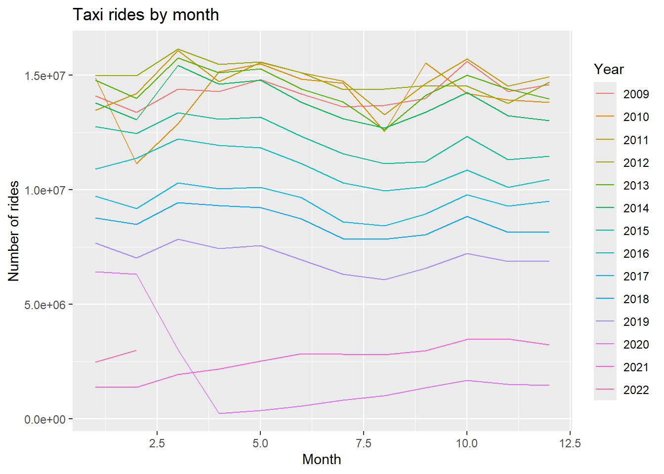
Lets do one more EDA, which months has highest counts of taxi rides.

## Count by year and month
df2 = ds %>% 
  count(year, month) %>% 
  collect()

## Plot
df2 %>% 
  ggplot(aes(x = month, y = n, color = factor(year))) +
  geom_line() +
  labs(title = "Taxi rides by month",
       x = "Month",
       y = "Number of rides",
       color = "Year")

Interesting trends that summer is lwoer and peaks consistent in october.

6.5 Summary

Parquet is a columnar storage format that is optimized for modern analytics
Arrow is a high performance data processing library that can work with parquet files in many languages
Arrow can work with parquet files out of memory and on distributed file systems
Arrow can work with parquet files on cloud storage such as AWS S3 and GCS
This workflow can enable data teams to work with large datasets on normal labtops and share data with external collaborators efficently, securely and scalably without any additiona infrastructure costs.